Using different diffusion coefficient datasets

By default, DiffusionGarnet.jl uses the diffusion coefficients of Chakraborty & Ganguly (1992) to model garnet diffusion. However, it is possible to use other datasets: the one from Carlson (2006) and the one from Chu and Ague 2015. This tutorial will show how to use these different datasets in DiffusionGarnet.jl and we will compare them with a simple simulation.

We will use the same data as in the 1D diffusion tutorial for this example. First, we will load the data, which should be in the same folder as your current session:

using DiffusionGarnet  # this can take a while
using DelimitedFiles
# load the data of your choice (here from the text file located in https://github.com/Iddingsite/DiffusionGarnet.jl/tree/main/examples/1D, place it in the same folder as where you are running the code)
data = DelimitedFiles.readdlm("Data_Grt_1D.txt", '\t', '\n', header=true)[1]

Mg0 = data[:, 4]  # load initial Mg mole fraction
Fe0 = data[:, 2]  # load initial Fe mole fraction
Mn0 = data[:, 3]  # load initial Mn mole fraction
Ca0 = data[:, 5]  # load initial Ca mole fraction
distance = data[:, 1]

Lx = (data[end,1] - data[1,1])u"µm"  # length in x of the model, here in µm
tfinal = 15u"Myr"  # total time of the model, here in Myr

# define the initial conditions in 1D of your problem
IC1D = IC1DMajor(;CMg0, CFe0, CMn0, Lx, tfinal)

# define the pressure and temperature conditions of diffusion
T = 700u"°C"
P = 0.6u"GPa"

To choose the diffusion coefficient dataset, it only requires a keyword argument in the Domain constructor: diffcoef.

It can take the following values:

• :C92 for the dataset of Chakraborty and Ganguly (1992), which is the default value.
• :C06 for the dataset of Carlson (2006)
• :CA15 for the dataset of Chu and Ague (2015)

Let's define three domains with these different datasets:

domain1D_C92 = Domain(IC1D, T, P, diffcoef = :C92)
domain1D_C06 = Domain(IC1D, T, P, diffcoef = :C06)
domain1D_CA15 = Domain(IC1D, T, P, diffcoef = :CA15)

We can now simulate the three domains:

sol_C92 = simulate(domain1D_C92; progress=true, progress_steps=1)
sol_C06 = simulate(domain1D_C06; progress=true, progress_steps=1)
sol_CA15 = simulate(domain1D_CA15; progress=true, progress_steps=1)

Done! We can now plot the results of our simulations to compare the different diffusion coefficient datasets:

# Choose consistent base colors for each element
col_Fe = 1
col_Mg = 2
col_Mn = 3
col_Ca = 4

anim = @animate for i in LinRange(0, sol_CG92.t[end], 100)
    l = @layout [a ; b]

    # ----------- Panel 1: Fe -----------
    p1 = plot(distance, CFe0, label="Fe initial",
              linestyle=:dash, linewidth=1, dpi=200,
              title=@sprintf("Total Time = %.2f Myr | T = %.0f °C | P = %.1f GPa",
                             i, T[1].val, P[1].val),
              legend=:outerbottomright, linecolor=col_Fe,
              xlabel="Distance (µm)")

    # Fe - CG92
    plot!(p1, distance, sol_CG92(i)[:,2], label="Fe CG92",
          color=col_Fe, linewidth=1, linestyle=:solid)
    # Fe - C06
    plot!(p1, distance, sol_C06(i)[:,2],
          label="Fe C06", color=col_Fe, linewidth=1, linestyle=:dashdot)
    # Fe - CA15
    plot!(p1, distance, sol_CA15(i)[:,2],
          label="Fe CA15", color=col_Fe, linewidth=1, linestyle=:dot)


    # ----------- Panel 2: Mg, Mn, Ca -----------
    p2 = plot(distance, CMg0, label="Mg initial",
              linestyle=:dash, linewidth=1, dpi=200,
              legend=:outerbottomright, color=col_Mg, xlabel="Distance (µm)")

    plot!(p2, distance, CMn0, label="Mn initial",
          linestyle=:dash, linewidth=1, color=col_Mn)
    plot!(p2, distance, CCa0, label="Ca initial",
          linestyle=:dash, linewidth=1, color=col_Ca)

    # Mg
    plot!(p2, distance, sol_CG92(i)[:,1], label="Mg CG92",
          color=col_Mg, linewidth=1, linestyle=:solid)
    plot!(p2, distance, sol_C06(i)[:,1],
          label="Mg C06", color=col_Mg, linewidth=1, linestyle=:dashdot)
    plot!(p2, distance, sol_CA15(i)[:,1],
          label="Mg CA15", color=col_Mg, linewidth=1, linestyle=:dot)

    # Mn
    plot!(p2, distance, sol_CG92(i)[:,3], label="Mn CG92",
          color=col_Mn, linewidth=1, linestyle=:solid)
    plot!(p2, distance, sol_C06(i)[:,3],
          label="Mn C06", color=col_Mn, linewidth=1, linestyle=:dashdot)
    plot!(p2, distance, sol_CA15(i)[:,3],
          label="Mn CA15", color=col_Mn, linewidth=1, linestyle=:dot)

    # Ca (closure relation)
    plot!(p2, distance, 1 .- sol_CG92(i)[:,1] .- sol_CG92(i)[:,2] .- sol_CG92(i)[:,3],
          label="Ca CG92", color=col_Ca, linewidth=1, linestyle=:solid)
    plot!(p2, distance, 1 .- sol_C06(i)[:,1]
                       .- sol_C06(i)[:,2]
                       .- sol_C06(i)[:,3],
          label="Ca C06", color=col_Ca, linewidth=1, linestyle=:dashdot)
    plot!(p2, distance, 1 .- sol_CA15(i)[:,1]
                       .- sol_CA15(i)[:,2]
                       .- sol_CA15(i)[:,3],
          label="Ca CA15", color=col_Ca, linewidth=1, linestyle=:dot)

    plot(p1, p2, layout=l)
end every 1

println("Now, generating the gif...")
gif(anim, "Grt_1D_compare.gif", fps = 7)
println("...Done!")

Here is the resulting gif obtained:

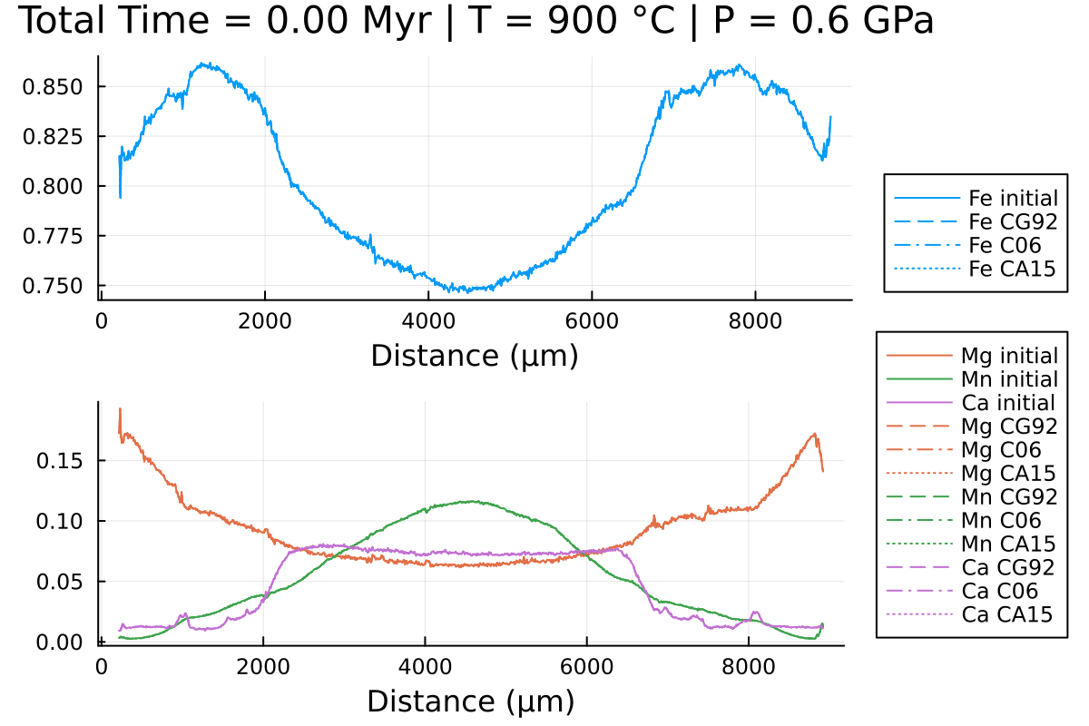
Notice the differences, especially in Mn and Fe.